Building a regression model for non-linear systems with Particle and Edge Impulse

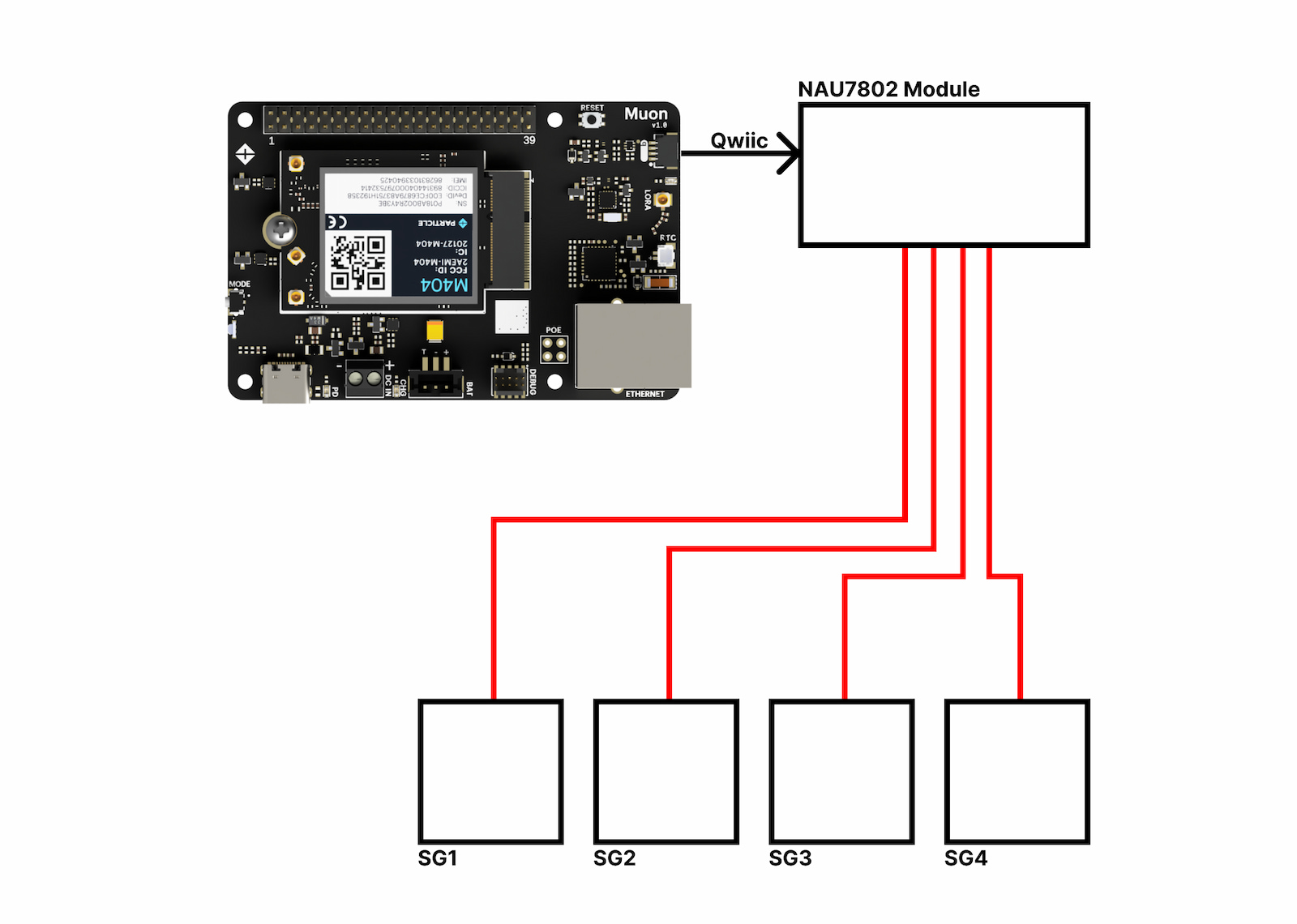
The Particle Muon with an M404 LTE SoM will be used as the data acquisition device. The M404 is plenty powerful enough to also run the trained regression model. The Muon provides a Qwiic connector, which allows for compatibility with a variety of off-the-shelf expansion modules. In this case, we’ll be using Adafruit’s NAU7802 ADC module to sample our four strain gauges configured in a wheatstone bridge configuration.

First, we’ll need to gather some training data. Prior research indicates that strain readings can be affected by temperature fluctuations and time. For this experiment we’ll just be focusing on the time component. We’ll use the difference of the known weight on the scale and the measured weight by the scale as the “label” in our dataset. The regression model will be responsible for estimating the measurement error. We’re trying to minimize the drift of the load cell over time therefore, our dataset should span many minutes or hours since the scale was last tare’d. This should allow the drift to accumulate. It would also be useful to have a variety of “known weights” on the scale so we can calculate the error at different loads.

The firmware for generating the training dataset is straight forward. More detail can be found in the GitHub repository. Our acquisition code logs the load cell reading and time_since_tare parameter over the serial port. There is also handling for incoming serial commands. t for tare, c for calibrate, and s for start. "Calibrate" requires a calibration weight parameter and "start" requires a known weight parameter (used in calculating the reading error).

#include "Particle.h"
#include "scale/scale.h"

SYSTEM_MODE(AUTOMATIC);

#define SYS_DELAY_MS 100

ScaleReading scaleReading = {0.0, 0};
char buf[128];

SerialLogHandler logHandler(
    LOG_LEVEL_NONE, // Default logging level for all categories
    {
        {"app", LOG_LEVEL_ALL} // Only enable all log levels for the application
    });

void setup()
{
  Serial.begin(115200);

  Particle.function("tare", tare);
  Particle.function("calibrate", calibrate);
  initializeScale();
}

float knownWeightValue = 0.0;

void loop()
{
  readScale(&scaleReading);
  unsigned long timeSinceTare = getTimeSinceTare();
  float error = knownWeightValue - scaleReading.weight;

  snprintf(buf, sizeof(buf), "%ld,%ld,%f,%f", timeSinceTare, scaleReading.raw, scaleReading.weight, error);
  Serial.println(buf);

  if (Serial.available() > 0)
  {
    String incomingString = Serial.readStringUntil('\n');
    incomingString.trim();
    String cmd = incomingString.substring(0, 1);
    String val = incomingString.substring(1);
    if (cmd == "t" || cmd == "T") // Tare the load cell and reset "time since tare"
    {
      tare("");
    }
    else if (cmd == "c" || cmd == "C") // Calibrate the load cell with a known weight
    {
      calibrate(val);
    }
    else if (cmd == "s" || cmd == "S") // Start the data collection and provide an expected weight
    {
      knownWeightValue = atof(val);
    }
  }
  delay(SYS_DELAY_MS);
}

A script written in Node.js will handle reading data from the serial port (the acquisition device) and appending it to a csv file. To run the script, clone the GitHub repository and open a terminal inside the project’s directory.

Then run:

npm install
node index.js

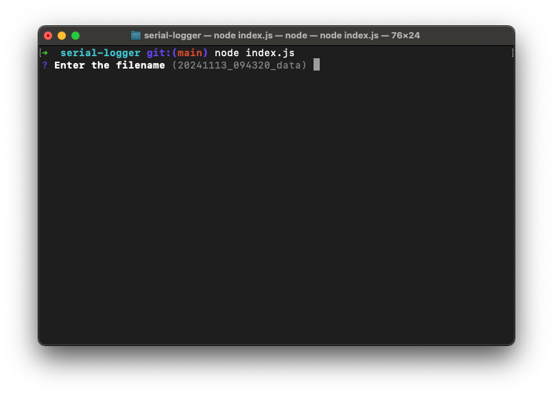
The program will start with a prompt for a filename for this dataset. You may chose to overwrite the default filename or press enter to accept the default.

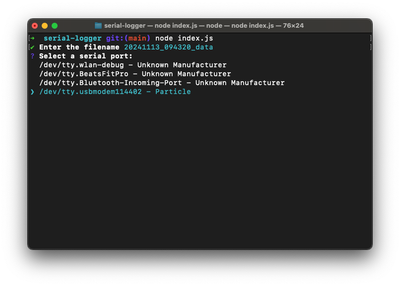
Next, you will be greeted with a serial port picker, select the port that is connected to a Particle device running the data acquisition firmware.

The script will now start printing serial data with the prefix of "not logging". This allows us to perform a couple of operations before recording the training data. Begin by tare’ing the scale to zero out the readings.

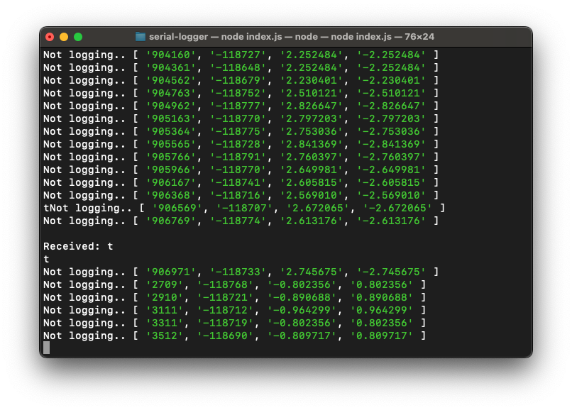
Then, if you haven’t done so already, type c <known weight value> + enter to calibrate the scale. This will only need to be done once as the calibration factor is saved to persistent memory.

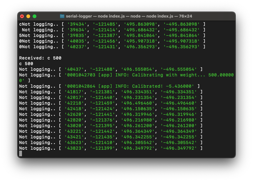
To start the logging process, type: s <known weight value> + enter. The program will then begin saving readings to the csv file. It will calculate the error (our dataset label) based on the known weight we just entered.

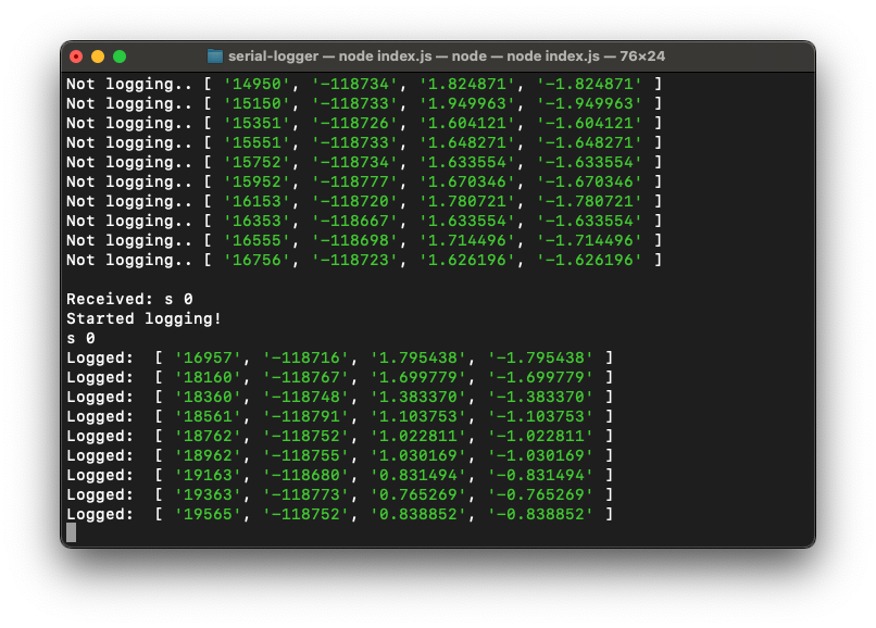
Gather a number of different datasets with varying "time since tare" values to demonstrate how the scale reading might change over time. It is important to note that resetting the device will always require another tare operation.

Add a few different known weights to the scale and re-do the data gathering with a range of "time since tare" windows.

Once we’re satisfied with our dataset, we can move on to the Edge Impulse model training step.

Let’s start training our regression model with the data we’ve just gathered. Navigate to Edge Impulse studio, create an account or log in, and create a new project. Select “Data acquisition” and “CSV Wizard” to begin importing our dataset.

Upload any csv file from the dataset gathered using the serial-logger program. In Step 2, accept the default delimiter.

For step 3, tell Edge Impulse that we are working with time-series data and choose the first formatting option.

Towards the bottom, configure the time step in milliseconds and override any abnormal timestamp differences.

In step 4, tell the wizard that raw_error contains the label you want to predict and include raw and raw_weight columns in your value set.

Finally, in step 5, limit your window to a specified window and choose the option to use the last value as the label for each sample. Essentially we’re assuming that the error won’t vary too dramatically in a 10 second window. We assume that we can use the last error reading as an estimate for the general error over the previous 10 seconds.

Upload the remaining CSV files in your training dataset after the wizard completes.

Navigate to the “Create Impulse” page and select a Particle device when prompted for a target. The following impulse design is what I found most accurate, but feel free to experiment.

Choose “Save Impulse” and navigate to the “Raw Data” page. Leave the defaults and click “Save parameters”. On the following page click “Generate features”.

Once the features have been generated, move on to the “Regression” page. I found success by updating the number of training cycles to 1000, but feel free to experiment. Click “Save & train” to start the model training process.

Once the model is trained head over to “Model testing” to get an idea of how your model performs against the test dataset.

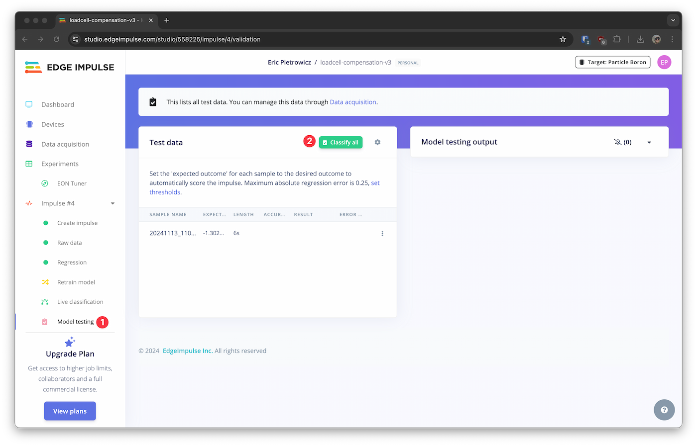
After the job completes, the results section will give you an idea of how well the model performs.

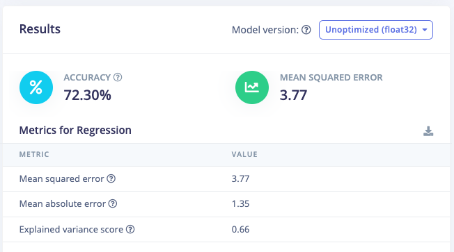
In this case our model is inferencing load cell error within 1.65 grams, 72% of the time. I’d say that is a pretty good result with minimal training data!

Now we can deploy the regression model to our hardware. Navigate to the deployment page and search for the Particle Library option. Keep the remaining default settings and choose “Build” at the bottom of the page.

Once the job completes, you’ll get a compressed folder containing your firmware with the compiled model.

Open the compiled firmware and modify the main.cpp file with the following code. Make sure to include the scale driver from the data acquisition sample. The full inference code can also be found in the GitHub repository. The modified code will maintain a rolling buffer of scale readings. The buffer then gets passed to the classifier to record predict the error. We can modify the calculated weight with the predicted error with the hope of improving our scale’s accuracy.

#include "Particle.h"
#include "scale/scale.h"
#include <loadcell-compensation-v2_inferencing.h>

SYSTEM_MODE(AUTOMATIC);

#define SYS_DELAY_MS 100

ScaleReading scaleReading = {0.0, 0};
char buf[128];

SerialLogHandler logHandler(LOG_LEVEL_ERROR);

/* Forward declerations ---------------------------------------------------- */
int raw_feature_get_data(size_t offset, size_t length, float *out_ptr);
void setup();
void loop();

static float features[EI_CLASSIFIER_DSP_INPUT_FRAME_SIZE];

/**
 * @brief      Copy raw feature data in out_ptr
 *             Function called by inference library
 *
 * @param[in]  offset   The offset
 * @param[in]  length   The length
 * @param      out_ptr  The out pointer
 *
 * @return     0
 */
int raw_feature_get_data(size_t offset, size_t length, float *out_ptr)
{
    memcpy(out_ptr, features + offset, length * sizeof(float));
    return 0;
}

void print_inference_result(ei_impulse_result_t result);

/**
 * @brief      Particle setup function
 */
void setup()
{
    // put your setup code here, to run once:

    // Wait for serial to make it easier to see the serial logs at startup.
    waitFor(Serial.isConnected, 15000);
    delay(2000);

    ei_printf("Edge Impulse inference runner for Particle devices\r\n");

    for (int i = 0; i < EI_CLASSIFIER_DSP_INPUT_FRAME_SIZE; i++)
    {
        features[i] = 0.0;
    }
}

/**
 * @brief      Particle main function
 */

int idx = 0;
float knownWeightValue = 0.0;
void loop()
{
    readScale(&scaleReading);
    unsigned long timeSinceTare = getTimeSinceTare();
    features[idx] = scaleReading.weight;
    idx = (idx + 1) % EI_CLASSIFIER_DSP_INPUT_FRAME_SIZE;

    if (Serial.available() > 0)
    {
        String incomingString = Serial.readStringUntil('\n');
        incomingString.trim();
        String cmd = incomingString.substring(0, 1);
        String val = incomingString.substring(1);
        if (cmd == "t" || cmd == "T")
        {
            tare("");
        }
        else if (cmd == "c" || cmd == "C")
        {
            calibrate(val);
        }
        else if (cmd == "s" || cmd == "S") // Start the data collection and provide an expected weight
        {
            knownWeightValue = atof(val);
        }
    }

    if (sizeof(features) / sizeof(float) != EI_CLASSIFIER_DSP_INPUT_FRAME_SIZE)
    {
        ei_printf("The size of your 'features' array is not correct. Expected %d items, but had %d\n",
                  EI_CLASSIFIER_DSP_INPUT_FRAME_SIZE, sizeof(features) / sizeof(float));
        return;
    }

    ei_impulse_result_t result = {0};

    // the features are stored into flash, and we don't want to load everything into RAM
    signal_t features_signal;
    features_signal.total_length = sizeof(features) / sizeof(features[0]);
    features_signal.get_data = &raw_feature_get_data;

    // invoke the impulse
    EI_IMPULSE_ERROR res = run_classifier(&features_signal, &result, false);
    if (res != EI_IMPULSE_OK)
    {
        ei_printf("ERR: Failed to run classifier (%d)\n", res);
        return;
    }
    float compensated_weight = scaleReading.weight + result.classification[0].value;
    float compensated_error = knownWeightValue - compensated_weight;
    float raw_error = knownWeightValue - scaleReading.weight;
    snprintf(buf, sizeof(buf), "%ld,%ld,%f,%f,%f,%f", timeSinceTare, scaleReading.raw, scaleReading.weight, raw_error, compensated_weight, compensated_error);
    Serial.println(buf);

    delay(SYS_DELAY_MS);
}

void print_inference_result(ei_impulse_result_t result)
{
    ei_printf("Timing: DSP %d ms, inference %d ms, anomaly %d ms\r\n",
              result.timing.dsp,
              result.timing.classification,
              result.timing.anomaly);

    ei_printf("Predictions:\r\n");
    for (uint16_t i = 0; i < EI_CLASSIFIER_LABEL_COUNT; i++)
    {
        ei_printf("  %s: ", ei_classifier_inferencing_categories[i]);
        ei_printf("%.5f\r\n", result.classification[i].value);
    }
}

Note that the Edge Impulse library includes references to Particle libraries that our not needed for our application. To fix this, go to project.properties and update it as follows:

name=<Your project's name>
version=1.0.4
author=<Your name>

Make sure to configure the project for your Particle device.

Now compile and flash the project!

The compensated data can be gathered by using a slightly modified version of the serial-logging script. Changes are made to include compensated_weight and compensated_error in the stored csv files. The files are then imported into a spreadsheet program and charted. By examining the charts we can see that, although error might slightly increase with short time_since_tare values, over a longer window sensor drift is meaningfully reduced.

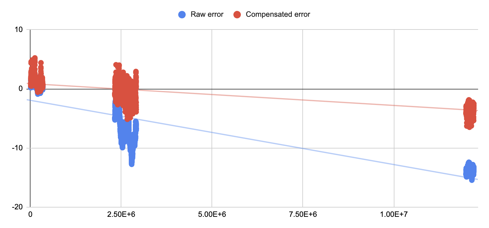
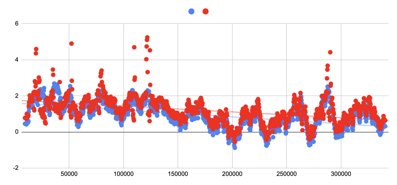
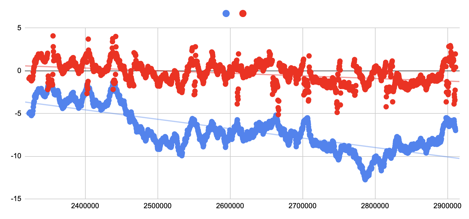
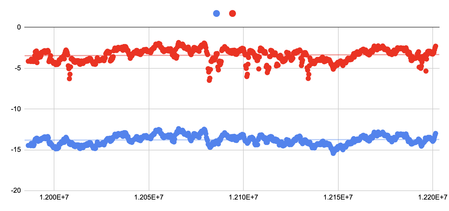
By including training data with additional weights, sampling over longer periods, or by including temperature and humidity readings our model could be improved. This post illustrates how to configure a non-discrete approach to a problem that is typically solved by discrete means. As your system increases in complexity, an inference model, such as the regression model detailed here, should be a tool to consider.